原子軌道の例
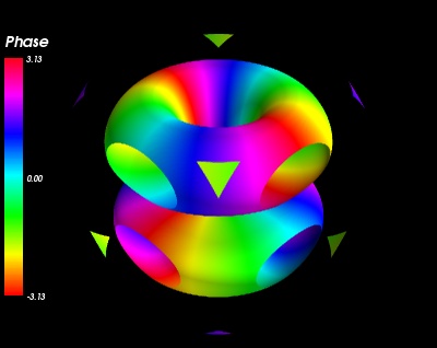
原子軌道のノルムと位相を示す例:ノルムの等値面と位相を示す色.
この例では,1つのデータセットにフィルタを適用し,フィルタの出力に2番目のデータセットを表示する方法を示します.ここでは,複素場のノルムの等値面を抽出するために輪郭フィルタを使用し,カラーマップにより場の位相を表示しました.
プロットするために選んだ場は,水素様原子の3P_y原子軌道を単純化したものです.
最初の手順は,2つのスカラーデータセットを持つデータソースを作成することです.次に, 'set_active_attribute' フィルタを使用してフィルタとモジュールを適用するデータを選択します.
2つのスカラーデータセットを使用してデータソースを作成するには,TVTKのデータセットのレイアウトをある程度理解する必要があるため,実際には少し面倒です.詳細については, Mayaviでのデータ表現 を参照してください.
Pythonソースコード: atomic_orbital.py
# Author: Gael Varoquaux <gael.varoquaux@normalesup.org>
# Copyright (c) 2008, Enthought, Inc.
# License: BSD Style.

# Create the data ############################################################
import numpy as np

x, y, z = np.ogrid[- .5:.5:200j, - .5:.5:200j, - .5:.5:200j]
r = np.sqrt(x ** 2 + y ** 2 + z ** 2)


# Generalized Laguerre polynomial (3, 2)
L = - r ** 3 / 6 + 5. / 2 * r ** 2 - 10 * r + 6

# Spherical harmonic (3, 2)
Y = (x + y * 1j) ** 2 * z / r ** 3

Phi = L * Y * np.exp(- r) * r ** 2

# Plot it ####################################################################
from mayavi import mlab
mlab.figure(1, fgcolor=(1, 1, 1), bgcolor=(0, 0, 0))
# We create a scalar field with the module of Phi as the scalar
src = mlab.pipeline.scalar_field(np.abs(Phi))

# And we add the phase of Phi as an additional array
# This is a tricky part: the layout of the new array needs to be the same
# as the existing dataset, and no checks are performed. The shape needs
# to be the same, and so should the data. Failure to do so can result in
# segfaults.
src.image_data.point_data.add_array(np.angle(Phi).T.ravel())
# We need to give a name to our new dataset.
src.image_data.point_data.get_array(1).name = 'angle'
# Make sure that the dataset is up to date with the different arrays:
src.update()

# We select the 'scalar' attribute, ie the norm of Phi
src2 = mlab.pipeline.set_active_attribute(src,
                                    point_scalars='scalar')

# Cut isosurfaces of the norm
contour = mlab.pipeline.contour(src2)

# Now we select the 'angle' attribute, ie the phase of Phi
contour2 = mlab.pipeline.set_active_attribute(contour,
                                    point_scalars='angle')

# And we display the surface. The colormap is the current attribute: the phase.
mlab.pipeline.surface(contour2, colormap='hsv')

mlab.colorbar(title='Phase', orientation='vertical', nb_labels=3)

mlab.show()