タンパク質の例
タンパク質データベースからダウンロードしたタンパク質グラフ構造を標準のpdbフォーマットで表示します.
ここではpdbファイルを構文解析しますが,原子のタイプ,原子の位置,原子間のリンクなど,非常に少量の情報しか抽出しません.
この例の複雑さの大部分は,PDB情報を,関連付けられたスカラーおよび接続情報とともに3D位置のリストに変換するコードに起因します.
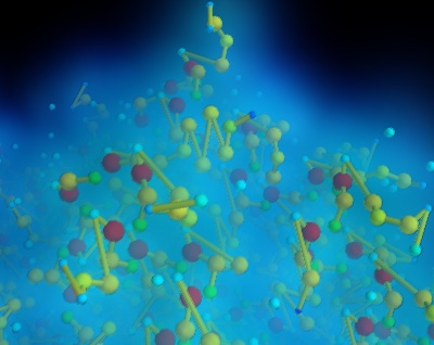
異なるタイプの原子を区別するために原子にスカラー値を割り当てたが,原子質量に対応しませんでした.したがって,可視化された原子の大きさと色は化学的に重要ではありません.
mlabを用いて原子をプロットしました. points3d および原子間の接続がデータセットに追加され,サーフェスモジュールを使用して視覚化されます.
グラフは,ポイントに接続情報を追加することによって作成されます.このために,各ポイントを番号( mlab.points3d に渡された配列順)で指定し,これらの番号の組からなる接続配列を構築する.pdbファイルに格納されている名前付きノードのグラフ表現からインデックスベースの接続ペアに移行するには,多少面倒なデータ操作があります.グラフをプロットする同様の手法は フライトグラフの例 で行われていますが,グラフをプロットする別の手法を示すグラフプロットの例が Delaunayグラフの例 で見られます.
局所原子密度を可視化するために,連続密度場のカーネル密度推定を構築するGaussスプラッターフィルタを使用しました.各点はGaussカーネルによって畳み込まれ,これらのGaussiansの和は結果として生じる密度場を形成します.このフィールドはボリュームレンダリングを使用して表示します.
pdbファイル標準のリファレンス: http://mmcif.pdb.org/dictionaries/pdb-correspondence/pdb2mmcif.html
Pythonソースコード: protein.py
# Author: Gael Varoquaux <gael.varoquaux@normalesup.org>
# Copyright (c) 2008-2020, Enthought, Inc.
# License: BSD Style.

# The pdb code for the protein.
protein_code = '2q09'

# Retrieve the file from the protein database #################################
import os
if not os.path.exists('pdb%s.ent.gz' % protein_code):
    # Download the data
    try:
        from urllib import urlopen
    except ImportError:
        from urllib.request import urlopen
    print('Downloading protein data, please wait')
    opener = urlopen(
      'ftp://ftp.wwpdb.org/pub/pdb/data/structures/divided/pdb/q0/pdb%s.ent.gz'
      % protein_code)
    open('pdb%s.ent.gz' % protein_code, 'wb').write(opener.read())

# Parse the pdb file ##########################################################
import gzip
infile = gzip.GzipFile('pdb%s.ent.gz' % protein_code, 'rb')

# A graph represented by a dictionary associating nodes with keys
# (numbers), and edges (pairs of node keys).
nodes = dict()
edges = list()
atoms = set()

# Build the graph from the PDB information
last_atom_label = None
last_chain_label = None
for line in infile:
    line = line.split()
    if line[0] in ('ATOM', 'HETATM'):
        nodes[line[1]] = (line[2], line[6], line[7], line[8])
        atoms.add(line[2])
        chain_label = line[5]
        if chain_label == last_chain_label:
            edges.append((line[1], last_atom_label))
        last_atom_label = line[1]
        last_chain_label = chain_label
    elif line[0] == 'CONECT':
        for start, stop in zip(line[1:-1], line[2:]):
            edges.append((start, stop))

atoms = list(atoms)
atoms.sort()
atoms = dict(zip(atoms, range(len(atoms))))

# Turn the graph into 3D positions, and a connection list.
labels = dict()

x = list()
y = list()
z = list()
scalars = list()

for index, label in enumerate(nodes):
    labels[label] = index
    this_scalar, this_x, this_y, this_z = nodes[label]
    scalars.append(atoms[this_scalar])
    x.append(float(this_x))
    y.append(float(this_y))
    z.append(float(this_z))

connections = list()

for start, stop in edges:
    connections.append((labels[start], labels[stop]))

import numpy as np
x = np.array(x)
y = np.array(y)
z = np.array(z)
scalars = np.array(scalars)

# Visualize the data ##########################################################
from mayavi import mlab
mlab.figure(1, bgcolor=(0, 0, 0))
mlab.clf()

pts = mlab.points3d(x, y, z, 1.5 * scalars.max() - scalars,
                                    scale_factor=0.015, resolution=10)
pts.mlab_source.dataset.lines = np.array(connections)

# Use a tube fiter to plot tubes on the link, varying the radius with the
# scalar value
tube = mlab.pipeline.tube(pts, tube_radius=0.15)
tube.filter.radius_factor = 1.
tube.filter.vary_radius = 'vary_radius_by_scalar'
mlab.pipeline.surface(tube, color=(0.8, 0.8, 0))

# Visualize the local atomic density
mlab.pipeline.volume(mlab.pipeline.gaussian_splatter(pts))

mlab.view(49, 31.5, 52.8, (4.2, 37.3, 20.6))

mlab.show()