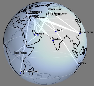
フライトグラフの例
地表に配置された都市間のグラフ表示の例.
このグラフは,Boing777が運用している最長飛行ルートを示しています.この例の主な目的は,任意の接続性のグラフを作成する方法と,地球の表面にデータを配置する方法を示すことです.
グラフを作成するには,まず mlab.points3d コマンドを使用してスカラ分散データセットを構築し,ライン情報を追加します.困難な点の一つは,点のインデックス番号を使用して行が指定されるため,ロード時にデータを 'massage' する必要があることです.グラフをプロットする同様のテクニックは タンパク質の例 で行われます.グラフをプロットする別の手法を示すグラフプロットの別の例は, Delaunayグラフの例 できます.
単純化するために,私たちは地球の表面に接続を描くのではなく,地球を通る直線として描きます.そのため,接続を表示するには透過性を使用する必要があります.
データソース: http://www.777fleetpage.com/777fleetpage3.htm
Pythonソースコード: flight_graph.py
###############################################################################
# The data. This could be loaded from a file, or scraped from a website

routes_data = """
Bombay,Atlanta
Johannesburg,Atlanta
Dubai,Los Angeles
Dubai,Houston
Dubai,San Francisco
New York,Hong Kong
Newark,Hong Kong
Doha,Houston
Toronto,Hong Kong
Bombay,Newark
Bombay,New York
Vancouver,Hong Kong
Dubai,Sao Paulo
Los Angeles,Sydney
Chicago,Delhi
"""

cities_data = """
Toronto,-79.38,43.65
Chicago,-87.68,41.84
Houston,-95.39,29.77
New York,-73.94,40.67
Vancouver,-123.13,49.28
Los Angeles,-118.41,34.11
San Francisco,-122.45,37.77
Atlanta,-84.42,33.76
Dubai,55.33,25.27
Sydney,151.21,-33.87
Hong Kong,114.19,22.38
Bombay,72.82,18.96
Delhi,77.21,28.67
Newark,-82.43,40.04
Johannesburg,28.04,-26.19
Doha,51.53,25.29
Sao Paulo,-46.63,-23.53
"""

###############################################################################
# Load the data, and put it in data structures we can use
import csv
routes_table = [i for i in csv.reader(routes_data.split('\n')[1:-1])]

# Build a dictionnary returning GPS coordinates for each city
cities_coord = dict()
for line in list(csv.reader(cities_data.split('\n')))[1:-1]:
    name, long_, lat = line
    cities_coord[name] = (float(long_), float(lat))

# Store all the coordinates of connected cities in a list also keep
# track of which city corresponds to a given index in the list. The
# connectivity information is specified as connecting the i-th point
# with the j-th.
cities = dict()
coords = list()
connections = list()
for city1, city2 in routes_table[1:-1]:
    if not city1 in cities:
        cities[city1] = len(coords)
        coords.append(cities_coord[city1])
    if not city2 in cities:
        cities[city2] = len(coords)
        coords.append(cities_coord[city2])
    connections.append((cities[city1], cities[city2]))


###############################################################################
from mayavi import mlab
mlab.figure(1, bgcolor=(0.48, 0.48, 0.48), fgcolor=(0, 0, 0),
               size=(400, 400))
mlab.clf()

###############################################################################
# Display points at city positions
import numpy as np
coords = np.array(coords)
# First we have to convert latitude/longitude information to 3D
# positioning.
lat, long = coords.T * np.pi / 180
x = np.cos(long) * np.cos(lat)
y = np.cos(long) * np.sin(lat)
z = np.sin(long)

points = mlab.points3d(x, y, z,
                     scale_mode='none',
                     scale_factor=0.03,
                     color=(0, 0, 1))

###############################################################################
# Display connections between cities
connections = np.array(connections)
# We add lines between the points that we have previously created by
# directly modifying the VTK dataset.
points.mlab_source.dataset.lines = connections
points.mlab_source.reset()
# To represent the lines, we use the surface module. Using a wireframe
# representation allows to control the line-width.
mlab.pipeline.surface(points, color=(1, 1, 1),
                              representation='wireframe',
                              line_width=4,
                              name='Connections')

###############################################################################
# Display city names
for city, index in cities.items():
    label = mlab.text(x[index], y[index], city, z=z[index],
                      width=0.016 * len(city), name=city)
    label.property.shadow = True

###############################################################################
# Display continents outline, using the VTK Builtin surface 'Earth'
from mayavi.sources.builtin_surface import BuiltinSurface
continents_src = BuiltinSurface(source='earth', name='Continents')
# The on_ratio of the Earth source controls the level of detail of the
# continents outline.
continents_src.data_source.on_ratio = 2
continents = mlab.pipeline.surface(continents_src, color=(0, 0, 0))

###############################################################################
# Display a semi-transparent sphere, for the surface of the Earth

# We use a sphere Glyph, through the points3d mlab function, rather than
# building the mesh ourselves, because it gives a better transparent
# rendering.
sphere = mlab.points3d(0, 0, 0, scale_mode='none',
                                scale_factor=2,
                                color=(0.67, 0.77, 0.93),
                                resolution=50,
                                opacity=0.7,
                                name='Earth')

# These parameters, as well as the color, where tweaked through the GUI,
# with the record mode to produce lines of code usable in a script.
sphere.actor.property.specular = 0.45
sphere.actor.property.specular_power = 5
# Backface culling is necessary for more a beautiful transparent
# rendering.
sphere.actor.property.backface_culling = True

###############################################################################
# Plot the equator and the tropiques
theta = np.linspace(0, 2 * np.pi, 100)
for angle in (- np.pi / 6, 0, np.pi / 6):
    x = np.cos(theta) * np.cos(angle)
    y = np.sin(theta) * np.cos(angle)
    z = np.ones_like(theta) * np.sin(angle)

    mlab.plot3d(x, y, z, color=(1, 1, 1),
                        opacity=0.2, tube_radius=None)

mlab.view(63.4, 73.8, 4, [-0.05, 0, 0])
mlab.show()