Mriの例

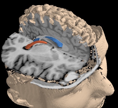
切断面と等値面を使用してMRIデータを表示します．

次の使用例は，MRIスキャンをダウンロードし，3D配列に変換して視覚化します．

まず脳の内部構造を抽出するために，その周囲の関心領域を定義し，等値面を用いました．

次に，2つの切断面を表示して，生のMRIデータ自体を示します．

最後に，外側サーフェスを表示しますが，切断面のカットを残すために，対象のボリュームに制限します．

Mayaviおよびvtkを使用したMRIデータからの特徴抽出の例については， Tvtkセグメンテーションの例 を参照のこと．

Pythonソースコード: mri.py

### Download the data, if not already on disk #################################
import os
if not os.path.exists('MRbrain.tar.gz'):
    # Download the data
    try:
        from urllib import urlopen
    except ImportError:
        from urllib.request import urlopen
    print("Downloading data, Please Wait (7.8MB)")
    opener = urlopen(
                'http://graphics.stanford.edu/data/voldata/MRbrain.tar.gz')
    open('MRbrain.tar.gz', 'wb').write(opener.read())

# Extract the data
import tarfile
tar_file = tarfile.open('MRbrain.tar.gz')
try:
    os.mkdir('mri_data')
except:
    pass
tar_file.extractall('mri_data')
tar_file.close()


### Read the data in a numpy 3D array #########################################
import numpy as np
data = np.array([np.fromfile(os.path.join('mri_data', 'MRbrain.%i' % i),
                                        dtype='>u2') for i in range(1, 110)])
data.shape = (109, 256, 256)
data = data.T

# Display the data ############################################################
from mayavi import mlab

mlab.figure(bgcolor=(0, 0, 0), size=(400, 400))

src = mlab.pipeline.scalar_field(data)
# Our data is not equally spaced in all directions:
src.spacing = [1, 1, 1.5]
src.update_image_data = True


# Extract some inner structures: the ventricles and the inter-hemisphere
# fibers. We define a volume of interest (VOI) that restricts the
# iso-surfaces to the inner of the brain. We do this with the ExtractGrid
# filter.
blur = mlab.pipeline.user_defined(src, filter='ImageGaussianSmooth')
voi = mlab.pipeline.extract_grid(blur)
voi.trait_set(x_min=125, x_max=193, y_min=92, y_max=125, z_min=34, z_max=75)

mlab.pipeline.iso_surface(voi, contours=[1610, 2480], colormap='Spectral')

# Add two cut planes to show the raw MRI data. We use a threshold filter
# to remove cut the planes outside the brain.
thr = mlab.pipeline.threshold(src, low=1120)
cut_plane = mlab.pipeline.scalar_cut_plane(thr,
                                plane_orientation='y_axes',
                                colormap='black-white',
                                vmin=1400,
                                vmax=2600)
cut_plane.implicit_plane.origin = (136, 111.5, 82)
cut_plane.implicit_plane.widget.enabled = False

cut_plane2 = mlab.pipeline.scalar_cut_plane(thr,
                                plane_orientation='z_axes',
                                colormap='black-white',
                                vmin=1400,
                                vmax=2600)
cut_plane2.implicit_plane.origin = (136, 111.5, 82)
cut_plane2.implicit_plane.widget.enabled = False

# Extract two views of the outside surface. We need to define VOIs in
# order to leave out a cut in the head.
voi2 = mlab.pipeline.extract_grid(src)
voi2.trait_set(y_min=112)
outer = mlab.pipeline.iso_surface(voi2, contours=[1776, ],
                                        color=(0.8, 0.7, 0.6))

voi3 = mlab.pipeline.extract_grid(src)
voi3.trait_set(y_max=112, z_max=53)
outer3 = mlab.pipeline.iso_surface(voi3, contours=[1776, ],
                                         color=(0.8, 0.7, 0.6))


mlab.view(-125, 54, 326, (145.5, 138, 66.5))
mlab.roll(-175)

mlab.show()

import shutil
shutil.rmtree('mri_data')