使用mlab配置pipeline管线

前面使用的绘图函数仅仅是Mayavi的一小部分，它还有更大的空间和可能性。Mayavi的全部威力需要配合pipeline管线才能完全释放出来。关于使用`data source`对象加载数据进行可视化可以参考章节`an-overview-of-mayavi`。其中有一个数据变换的环节是可选的：它通过`filters`滤波层级和`module`可视化层级完成。而mlab函数仅通过1行代码就能完成复杂的管线配置，完成sources数据源层级，filters层级以及module层级的搭建。其弊端是分化过于完全无法做更多的延伸，以及探索可能的结合方式。

Mlab所包含的子模块`pipeline` 可以使脚本能轻松配置管线。这个模块可以使用 `mlab`调用：`mlab.pipeline，或者直接以 `mayavi.tools.pipeline`方式引入环境。

当我们使用`mlab`绘图函数的时候，管线已会自动完成搭建：首先是来自`numpy`数组的数据创建source数据源层级，然后是module可视化模块层级，在两者之间可能带有filter滤波层级。对于已经配置好的管线，我们可以使用 `mlab.show_pipeline`进行查看。利用它的层级配置信息，我们可以使用`pipeline`的配置方法对其进行复现。在这里我们需要各个层级的配置函数的信息，其所使用的函数名默认也是pipeline管线的函数名。下面我们演示一个案例，使用`surf`函数构建可视化： 译者注：这是两种绘图的方式，前者是直接使用高度预制好的surf绘图函数，后者使用pipeline按层搭建，旨在说明两者具有相同的效果。比如Array2DSource数据源层级的名称，也是pipeline的方法名pipeline.array2d_source。

import numpy as np
a = np.random.random((4, 4))
from mayavi import mlab
mlab.surf(a)
mlab.show_pipeline()

以下是所创建的管线：

Array2DSource
    \__ WarpScalar
            \__ PolyDataNormals
                    \__ Colors and legends
                            \__ Surface

相同的pipeline管线也可以用下面的代码进行搭建：

src = mlab.pipeline.array2d_source(a)
warp = mlab.pipeline.warp_scalar(src)
normals = mlab.pipeline.poly_data_normals(warp)
surf = mlab.pipeline.surface(normals)

Data sources数据源层级

The mlab.pipeline module contains functions for creating various data sources from arrays. They are fully documented in details in the Mlab 管线配置参考. We give a small summary of the possibilities here.

Mayavi将数据区分为**scalar data 标量数据**和**vector data 矢量数据**。有一点尤为重要，他们用不同的方法创建**unconnected points 离散点**，或具有连续变化的**connected data points 连续点** 。后者会在点与点时间采用插值，在物理和工程上是`fields 场`的概念。

Unconnected sources:

scalar_scatter() (creates a PolyData)

vector_scatter() (creates an PolyData)

implicitly-connected sources:

scalar_field() (creates an ImageData) vector_field() (creates an ImageData)

array2d_source() (creates an ImageData)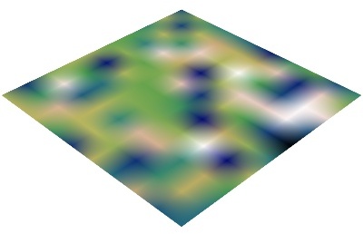

Explicitly-connected sources:

line_source() (creates an PolyData)

triangular_mesh_source() (creates an PolyData)

All the mlab.pipline source factories are functions that take numpy arrays and return the Mayavi source object that was added to the pipeline. However, the implicitly-connected sources require well-shaped arrays as arguments: the data is supposed to lie on a regular, orthogonal, grid of the same shape as the shape of the input array, in other words, the array describes an image, possibly 3 dimensional.

备注

More complicated data structures can be created, such as irregular grids or non-orthogonal grid. See the section on data structures.

Modules and filters

For each Mayavi module or filter (see Module 可视化模块 and Filters), there is a corresponding mlab.pipeline function. The name of this function is created by replacing the alternating capitals in the module or filter name by underscores. Thus ScalarCutPlane corresponds to scalar_cut_plane.

In general, the mlab.pipeline module and filter factory functions simply create and connect the corresponding object. However they can also contain addition logic, exposed as keyword arguments. For instance they allow to set up easily a colormap, or to specify the color of the module, when relevant. In accordance with the goal of the mlab interface to make frequent operations simple, they use the keyword arguments to choose the properties of the created object to suit the requirements. It can be thus easier to use the keyword arguments, when available, than to set the attributes of the objects created. For more information, please check out the docstrings. Full, detailed, usage examples are given in the next subsection.