化学の例

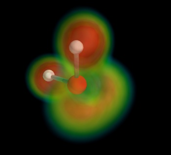
この例では，H2O分子を表示し，ボリュームレンダリングを使用して電子の局在化関数を表示します．

mlabを使用して原子と境界を表示します．色を制御するスカラー情報を持つmlab.points3dとmlab.plot3dです．

電子局在化関数はボリュームレンダリングを用いて表示される． mlab.pipeline.volume に vmin と vmax の引数をうまく使用することは，良い可視化を達成するために重要です． vmin 閾値は，特徴が際立つのに十分高い位置に置かれるべきである．

オリジナルはAxel Kohlmeyerの電子局在化関数である．

Pythonソースコード: chemistry.py

# Author: Gael Varoquaux <gael.varoquaux@normalesup.org>
# Copyright (c) 2008-2020, Enthought, Inc.
# License: BSD Style.

# Retrieve the electron localization data for H2O #############################
import os
if not os.path.exists('h2o-elf.cube'):
    # Download the data
    try:
        from urllib import urlopen
    except ImportError:
        from urllib.request import urlopen
    print('Downloading data, please wait')
    opener = urlopen(
        'http://code.enthought.com/projects/mayavi/data/h2o-elf.cube'
        )
    open('h2o-elf.cube', 'wb').write(opener.read())


# Plot the atoms and the bonds ################################################
import numpy as np
from mayavi import mlab
mlab.figure(1, bgcolor=(0, 0, 0), size=(350, 350))
mlab.clf()

# The position of the atoms
atoms_x = np.array([2.9, 2.9, 3.8]) * 40 / 5.5
atoms_y = np.array([3.0, 3.0, 3.0]) * 40 / 5.5
atoms_z = np.array([3.8, 2.9, 2.7]) * 40 / 5.5

O = mlab.points3d(atoms_x[1:-1], atoms_y[1:-1], atoms_z[1:-1],
                  scale_factor=3,
                  resolution=20,
                  color=(1, 0, 0),
                  scale_mode='none')

H1 = mlab.points3d(atoms_x[:1], atoms_y[:1], atoms_z[:1],
                   scale_factor=2,
                   resolution=20,
                   color=(1, 1, 1),
                   scale_mode='none')

H2 = mlab.points3d(atoms_x[-1:], atoms_y[-1:], atoms_z[-1:],
                   scale_factor=2,
                   resolution=20,
                   color=(1, 1, 1),
                   scale_mode='none')

# The bounds between the atoms, we use the scalar information to give
# color
mlab.plot3d(atoms_x, atoms_y, atoms_z, [1, 2, 1],
            tube_radius=0.4, colormap='Reds')

# Display the electron localization function ##################################

# Load the data, we need to remove the first 8 lines and the '\n'
str = ' '.join(file('h2o-elf.cube').readlines()[9:])
data = np.fromstring(str, sep=' ')
data.shape = (40, 40, 40)

source = mlab.pipeline.scalar_field(data)
min = data.min()
max = data.max()
vol = mlab.pipeline.volume(source, vmin=min + 0.65 * (max - min),
                                   vmax=min + 0.9 * (max - min))

mlab.view(132, 54, 45, [21, 20, 21.5])

mlab.show()